Theory of Advective Effects on Biological Dynamics II - Robinson
On the Theory of Advective Effects on
Biological Dynamics in the Sea II:
Localization, Light Limitation, and Nutrient
Saturation
Proceedings of the Royal Society A, 455, 1813-1828, 1999.
Allan R. Robinson
Division of Engineering and Applied Sciences,
Department of Earth and Planetary Sciences,
Harvard University, Cambridge, MA 01238, U.S.A.
robinson@pacific.harvard.edu
Abstract
The theory of advective effects is extended to include:
localization effects due both to the attenuation of light with
depth in the ocean, and to nutrient transport into the
euphotic zone of finite duration
in time, and/or over a limited horizontal domain.
Also nutrient
uptake is generalized to nonlinear Michaelis-Menten kinetics.
The characteristic curves are solved for
explicitly and a symbolic general solution
is obtained for arbitrary biological dynamics.
Some exemplary results are presented for the
effect of light, nutrient, and grazing
limitations on primary productivity in an NPZ-model.
The theory is now applicable to further
studies of more realistic oceanic processes.
In the following document, problems have been encountered translating TeX constructs
into HTML in text paragraphs. For example, the construct
in text can significantly affect line format and paragraph construction.
At present, this is unadvoidable and should be kept in mind while reading this
document.
1. Introduction
Interactive physical-biological dynamical processes
in the sea are of central importance to fundamental
and applied research in many areas of
interdisciplinary ocean science today,
including e.g., the dynamics of ecosystems
and biogeochemical cycles. Three major interactive
processes are physiological thermodynamics,
1 diffusion
and mixing, and advection. This study is focussed
on the advective process and attempts to
provide an idealized general theoretical framework for the
exploration of effects of various phenomenological
flow fields which occur in the ocean over a
broad range of time and space scales. It is
intended to complement related process
research based upon experimentation and simulation.
Additionally this theoretical approach may be of
some general interest for applications to
analogous problems of the reactive dynamics of
advected tracers in other fluids, e.g., in
chemical and engineering problems.
The first part of this study (Robinson, 1997)
introduced a biological dynamical model
consisting of growth, self-interaction and
bilinear interactions among n state
variables occurring in the presence of a
stretching deformation flow field. A general
theoretical approach via the theory of
characteristics was formulated and some
solutions were obtained for dynamical processes homogeneous in
space and impulsive in time. In this second
part, the nonlinear dynamics is extended
to include the Michaelis-Menten nonlinear
formulation for the uptake of nutrients
by phytoplankton. The ocean is divided
into an upper ocean where sunlight is
available for photosynthesis (euphotic
zone) and a deeper ocean which is not illuminated
(aphotic zone). Kinematical flow fields
are introduced which allow for the
localization of advective effects both horizontally
and in time. A general solution is
obtained for these kinematics and dynamics
and some idealized illustrative examples
presented. These developments should serve as the
basis for theoretical studies of realistic
oceanic processes.
Section 2 presents the model, section 3
solves for the characteristics and section 4
solves for the dynamics. Section 5
derives the general solution, section 6
provides examples and section 7
summarizes and concludes.
2. The model
The general model to be studied is that of equation (2.3) of part
I (which we will refer to as equation (I.2.3)) for
n biological state variables fi in two
spatial dimensions with diffusion neglected
|
|
¶fi
¶t
|
+u |
¶fi
¶x
|
+v |
¶fi
¶y
|
= Bi(f1,Ľ,fi,Ľ,fn) . (2.1) |
|
The flow field is specified kinematically in terms of a
stream function y(x,y,t) such that (vid. equation (I.2.9))
|
u = - |
¶y
¶y
|
v = |
¶y
¶x
|
, (2.2a) |
|
|
|
D fi
D t
|
ş |
¶fi
¶t
|
+u |
¶fi
¶x
|
+v |
¶fi
¶y
|
= |
¶fi
¶t
|
- |
¶y
¶y
|
|
¶fi
¶x
|
+ |
¶y
¶x
|
|
¶fi
¶y
|
, (2.2b) |
|
and the continuity equation ux+vy = 0 for mass
conservation in an almost incompressible Boussinesq
fluid (Tritton, 1988, Appendix to Ch. 14) is satisfied. The kinematics of
this section are
applicable to general biological dynamics Bi.
For the study of light limitation and to illustrate the
effects of flow kinematics on biological dynamics we
adopt the general NPZ-model of Part I section (4d), but
with Michaelis-Menten kinetics of nutrient uptake
and light attenuation
(Parsons et al., 1984;
Kirk, 1994). Then for phytoplankton (f1 = P),
zooplankton (f2 = Z) and nutrient (f3 = N), the
governing equations are (with reference to (I.2.10)
and (I.4.11)
where
|
U ş |
a13l(y)PN
K+N
|
. (2.3d) |
|
The independent variable 0 < y < Ą represents depth into the
ocean from the sea surface; l(y) is a nondimensional
light attenuation coefficient. The base of the euphotic
zone is located at y = ye with l(y > ye) ş 0.
The interaction coefficient a21 (dimensions
[l3(mt)-1] where m, l, t are units of
mass, length and time) is the zooplankton grazing rate;
a13([t-1]) is the phytoplankton maximum specific
rate of growth, and K ([ml-3]) is
the half saturation constant for nutrient uptake.
The dependent variables N,P,Z ([ml-3]) are all
dimensionalized by a biomass density M, where M is to be
chosen as a characteristic value of N advected into the
euphotic zone during any injection event of interest. The
independent variables (x,y,t)
are scaled respectively by (x0,y0 = ye,t0 = K(Ma13)-1)
where x0 is an horizontal length characterizing
a localized upwelling event. The horizontal and vertical
velocities (u,v) are scaled respectively by
(u0, v0 with u0 = v0x0y0-1), which yields a
nondimensional continuity equation ux+vy = 0. This
implies a scaling of y0 = u0y0 = v0x0.
The kinematical flow field is chosen such that the
horizontal velocity is independent of y and the product
of a function of x times a function of t. As in part I both
dimensional and nondimensional variables are represented by the
same symbols. Thus nondimensionally
|
y = -yf(t)g(x), u = fg, v = -yf |
dg
dx
|
(2.4a) |
|
|
|
D
Dt
|
= |
¶t
|
+ a |
é
ę
ë
|
- |
¶y
¶y
|
|
¶x
|
+ |
¶y
¶x
|
|
¶y
|
ů
ú
ű
|
(2.4b) |
|
The three-nondimensional parameters characterizing advection
(a), grazing (b), and uptake kinetics (d)
are defined by
|
a ş |
v0t0
y0
|
= |
uot0
x0
|
= |
v0K
yea13 M
|
b ş a21t0 = |
a21K
a13M
|
d ş |
M
K
|
(2.4g) |
|
3. Kinematics and Characteristics
For the flow system given by the stream function of
equation (2.4a) the characteristic equations (I.2.12a) take the
form
|
|
dt
ds
|
= 1, |
dx
ds
|
= au = af(t)g(x), |
dy
ds
|
= av = -ay |
dg
dx
|
f, (3.1a,b,c) |
|
with initial conditions taken as 2
|
s = 0: t = p, x = r, y = q. (3.2) |
|
The set (3.1) can be solved by two exact integrals and
a quadrature. Integrating (3.1a) directly, and after equating
ds from (3.1b,c), we obtain
|
t = s+p, yg(x) = qg(r), (3.3a,b) |
|
and after equating ds from (3.1a,b)
|
G(x,r) = aF(t,p), G(x,r) ş |
ó
ő
|
x
r
|
|
dx˘
g(x˘)
|
, F(t,p) ş |
ó
ő
|
t
p
|
f(t˘) dt˘. (3.3c) |
|
The function f(t) is chosen so as to represent either i) a
steady-state flow (S) or ii) a time-periodic flow
with nondimensional frequency w, which over a
half-period may be taken to represent an advective event (E). Thus
|
S: f = 1, FS = t-p, (3.4a) |
|
|
E: f = sinwt, FE = |
1
w
|
[coswp-coswt]. (3.4b) |
|
Three flow forms are evaluated for the function
g(x): i) a simple stretching deformation (D)
as in part I of this study; ii) a localized
(exponentially decaying) deformation (L);
iii) a simply periodic wave form (W). Whence
|
D: g = x, xy = qr, GD = ln |
x
r
|
(3.4c) |
|
|
L: g = 1-e-x(x > 0), y(1-e-x) = q(1-e-r), GL = ln |
é
ę
ë
|
(ex-1)
(er-1)
|
ů
ú
ű
|
(3.4d) |
|
|
W: g = sinx, ysinx = qsinr, GW = ln |
é
ę
ę
ę
ę
ę
ę
ę
ę
ë
|
|
ů
ú
ú
ú
ú
ú
ú
ú
ú
ű
|
. (3.4e) |
|
Consider the half-plane
x > 0; then (3.4d)
provides a simple kinematical model for coastal upwelling.
To study an open ocean isolated and localized upwelling
the flow may be completed by g = -1+ex (x < 0). Similarly
(3.4e) represents a periodic pattern of upwelling and
downwelling cells. The upwelling region
can serve as a simple
two-dimensional kinematical model of a cyclonic (cold core)
eddy.
Two initial value problems in s are necessary to carry out the
dynamical studies of the next sections. We assume that light
penetrates, and biological activity occurs, only to the
base of the euphotic zone located at y = 1.
The first problem is the time initial value problem
(T) as in part I. The second problem is the boundary
value problem (B) which specifies the values of the state
variables as they are advected across the base of the euphotic
zone from the deeper aphotic
zone where l = 0. As will be seen below, the T problem
is relevant to the deep pure advection (TA), and to the biological
dynamics in the water located initially in the
upper euphotic zone (TE).
Most interestingly, the B problem describes
the biological activity, in the euphotic zone, of water
located initially below the euphotic zone.
Under equations (I.2.13) and (3.2)
|
T: when s = 0, t = 0; thus p = 0 and |
|
|
fi(x,y,0) ş fi0(x,y)Ţfi0(r,q) (3.5a) |
|
|
B: when s = 0, y = 1; thus q = 1 and |
|
|
fi(x,1,t) ş fi0(x,t)Ţfi0(r,p) (3.5b) |
|
The functions following the arrows indicate the forms
(vid. equations (I.2.13, 14, 15)) in which
the initial conditions will appear in the solutions to the
dynamical equations of the next section. The domain of
interest is restricted to positive y and t. Thus fi0(r,p) is defined only for p ł 0. This implies a boundary
(or front) located at
,
separating water initially (t = 0) above or below the
euphotic zone, which is advected upward towards the sea
surface in time. Thus the domain of the B problem is defined
by
|
|
^
y
|
< y < 1, where p( |
^
x
|
, |
^
y
|
, |
^
t
|
) ş 0. (3.5c) |
|
The domain of the TA problem is y > 1 and that of
TE is
.
Combining the space-time kinematics, i.e., solving
equations (3.3) with the structures of (3.4) yields
six flow fields summarized in Table 1. The twelve sets of
characteristic curves corresponding to the T and B
problems for each flow are presented in Table 2.
To study light limitation effects, it is necessary to
evaluate the light attenuation coefficient and its
integral in s, i.e., l(y) of equation
(2.3d) in terms of y(s; p,r,q) which is given in
Table 3.
The F(s,p) is obtained from equations (3.4a,b)
evaluated with t = s+p for the S and E flows;
p = 0 and q = 1 respectively for the T and B problems.
4. Biological Dynamics
The s-domain biological dynamics for the NPZ system to be studied
here satisfies the nondimensional equations
|
|
dP
ds
|
= |
l(y)NP
1+dN
|
-bPZ (4.1a) |
|
with first integral
|
N+P+Z ş B = N0+P0+Z0 (4.1d) |
|
since mortality has been neglected.
The presence of the light attenuation (l) and nutrient
saturation (d) parameters in addition to the
grazing parameter (b) generalize the NPZ system of
equations (I.4.11). To elucidate basic processes we shall
consider the dynamics of systems of one, two, and three
state variables.
(a) P Model
The Malthusian growth of phytoplankton with unlimited nutrient and
no predation (Z = 0) satisfies (4.1a) with d >> 1
|
P = P0e[(s)/(d)], s ş |
ó
ő
|
s
0
|
l(y(s˘;p,r,q)) (4.2) |
|
with reference to Table 3.
(b) N-P Model
We retain Z = 0, insert P from (4.1d) into (4.1c) and
integrate, whence
|
(B-N)1+dB = AN, A ş |
P01+dB
N0
|
eBs (4.3a) |
|
with s as in (4.2). For d = 0 the solutions are as in
equation (I.4.12i)
|
P = |
P0B
N0e-Bs+P0
|
N = |
N0Be-Bs
N0e-Bs+P0
|
. (4.3b) |
|
(c) N-P-Z Model
To continue analytically following the procedure of equations
(I.4.12a,b,c) it is necessary to restrict
consideration to a uniformly
illuminated euphotic zone overlying a deep completely
aphotic ocean, i.e.,
|
l = l0, 0 < y < 1; l = 0, 1 < y. (4.4) |
|
Without loss of generality we may set l0 = 1 by rescaling
the parameters of (2.4g), i.e., by replacing a13 by
l0 a13.
Then equating ds from (4.1b,c) yields another first integral
which together with (4.1d) reduces (4.1c) to quadrature, i.e.
|
|
ó
ő
|
|
(1+dN)dN
-N2+BN- CN (1-b)e-dbN
|
= -s. (4.5b) |
|
For the case of b = 1 we can generalize the results of
(I.4.12d,e) for dN Ł 1. Keeping three terms in the Taylor series
expansion of the exponential, the denominator of (4.5b)
becomes
|
- |
ć
ç
č
|
1+ |
Cd2
2
|
ö
÷
ř
|
N2+(B+Cd)N-C. (4.5c) |
|
Integration yields
|
E[-2cN-(b-d)](cN2+bN+a)1/2c = [2cN+b+d]e-D s (4.5d) |
|
where
|
a = -C b = B+Cd c = - |
ć
ç
č
|
1+C |
d2
2
|
ö
÷
ř
|
|
|
and E is a constant of integration. The three s-integration
constants (B,C,E) are evaluated at s = 0 from (N0,P0,Z0)
in terms of (x,y,t) which are then replaced throughout the
domain by (r,p,q). The case of d = 0 reduces
to (I.4.12d,e),
|
N = |
E(B-D)+(B+D)e-D s
2(E+e-Ds)
|
, D = (B2-4C)1/2 (4.5e) |
|
|
B = N0+P0+Z0 C = N0Z0 E = |
B+D-2N0
2N0-(B-D)
|
. |
|
5. General Solution
For the n state variables of equation (2.1), there are
n-dynamical equations
|
|
dfi
ds
|
= Bi(fj), i,j = 1,Ľ, n 0 < y < 1 (5.1a) |
|
to be solved together with the characteristics (3.1).
Recall the three regions introduced preceding
equation (3.5). The TE problem is an independent
time initial value problem, but the B problem is coupled
to the TA problem. For the characteristic solutions (Table 2)
we introduce both for the (s,r,p,q)
and fi variables a subscript a for the advective
aphotic zone (1 < y) and e for the dynamically
active euphotic zone
. Let
|
fia(x,y,0) ş fiao(x,y) . (5.2a) |
|
Then by (5.1b)
|
fia(x,y,t) = fiao(ra(x,y,t), qa(x,y,t)) , (5.2b) |
|
and at the base of the euphotic zone
|
fia(x,1,t) = fiao(ra(x,1,t), qa(x,1,t)) ş fieo(x,t) = fie(x,1,t) . (5.2c) |
|
Thus the initial condition functions for the solution of
(5.1a) in
are given by
|
fieo(re,pe) = fiao(ra(re,1,pe), qa(re,1,pe)) . (5.2d) |
|
The general solution to (5.1a) is expressed as
|
fie(x,y,t) = fie(se; fjeo(re,pe)) , j = 1Ľn (5.3a) |
|
with the fjeo as given by (5.2d).
Consider now the case of pure advection everywhere, i.e.,
set Bi = 0 in (5.1a). Then the advective solution (5.2b) is
valid also in
. Also, however, for pure advection the state
variables are uncoupled and the general solution (5.3a)
reduces to
|
fie(x,y,t) = fieo(re,pe) , (5.3b) |
|
i.e., to (5.2d). Since the advective solutions (5.2b)
and (5.2d) must be the same, the identities
|
ra(re,1,pe) = ra(x,y,t), qa(re,1,pe) = qa(x,y,t) (5.3c) |
|
must hold.
Thus the general solution (5.3a) with biological
dynamics has the final form
|
| |
|
|
= fie(se;fjao(ra(x,y,t),qa(x,y,t)) j = 1Ľn, |
|
| | or omitting subscripts | | |
|
= fi(s;fjo(r,q)), |
^
y
|
< y < 1. |
|
|
| |
|
At the base of the euphotic
zone y = 1 and s = 0. At the shoaling front
and
by (3.5c) and (3.3a).
6. Examples
The general results derived here are intended to provide
the basis for a number of theoretical studies relevant
to real ocean processes. Here we will simply
illustrate effects in terms of a few idealized
simple examples.
(a) Light Limitation
We will first consider the localization effects arising
from biological activity being restricted to the
euphotic zone, in terms of the time initial value
problem and deformation field flow of part I., i.e.,
the DSB and DST flows of Table 2. We assume initially no
nutrient in the euphotic zone but a reservoir of nutrient
and seed populations of plankton below the euphotic zone.
The TE problem is trivially advective.
For y ł 1 (5.2b)
takes the form, e.g.,
|
P(x,y,t) = P0(r,q) = P0(xe-at, yeat) (6.1a) |
|
and
equations (5.2c,d) become at y = 1
|
P(x,1,t) = P0(xe-at, eat ), P0(r,p) = P0(r |
_
e
|
ap
|
,eap). (6.1b) |
|
From Table 2
|
reap = xye-a[t-1/aln1/y] = xe-at, eap = yeat (6.1c) |
|
consistently with (5.3c); thus
|
P0(r,p) = P0(xe-at,yeat), (6.1d) |
|
and similarly for N0, Z0. From (3.5c) the advancing
front is given by
|
|
^
t
|
= |
1
a
|
ln |
1
|
or |
^
y
|
= e-a[^(t)], P0(x, |
^
y
|
, |
^
t
|
) = P0(xe-a[^(t)],1). (6.1e) |
|
The simplest example is the Malthusian growth of equation (4.2).
Without loss of generality we can set d = 1, i.e., by
replacing a13 in (2.4g) by d-1a13.
We consider two cases: i) uniform light; 3
ii) linearly decreasing light. Then
i)
| l = l0 , s = l0 s = |
l0
a
|
ln1/y , es = (1/y)[(l0)/(a)] ,
|
and
ii)
| l = 1-y , s = |
1
a
|
[ln1/y+(y-1)] , es = [1/y e(y-1)][1/(a)]
|
( i) and ii) comprise 6.2a)
For the case of no x-dependence, the solutions (4.2) are
i)
| P(y,t) = P0(yeat)(1/y)[(l0)/(a)] , P(1,t) = P0(eat) , |
P( |
^
y
|
,t) = P0(1)el0t
|
and
ii)
| P(y,t) = P0(yeat)[ 1/y e(y-1)][1/(a)] , P(1,t,) = P0(eat) , |
P( |
^
y
|
, t) = P0(1)et+[((e-at-1))/(a)].
|
( i) and ii) comprise 6.2b)
Consider first the case of a deep reservoir of seed
plankton which is independent of depth, P0 = 1. Then for
there is a steady state solution, since water
parcels reaching a given depth at any time have spent the same amount
of time in the euphotic zone. The shallowest parcels have spent
the longest time under illumination, resulting in the
simple exponential growth at
, independent of
a, for case (i). For short times and depths near unity
the two solutions are dominated by advection. If the time
interval of interest is
and
, then the
choice of an effective uniform illumination
equates
for the two cases.
Any criteria to determine an effective l0, e.g.,
integrated net production, must take into account the flow
(a) and duration
.
(b) Uniform Deep Reservoirs
We extend the case of uniform deep reservoirs
with DS flow to the two (2)
and three (3) state variables biological systems and consider
essentially a unit source of nutrient together with very
small amount(s) of background plankton(s). The solutions
retain the character of establishing a
steady state below a shoaling front. The
analytical solutions to equations (4.3a) and (4.5e) are
particularly simple with (2) B = 1, and (3) D = 1
respectively, which is achieved by choosing
|
\noindent (2): N0 = 1-e P0 = e << 1 B = 1 (6.3) |
|
|
\noindent (3): N0 = 1 P0 = e(1-e) Z0 = e(1+e) |
|
|
B = 1+2e C = e(1+e) D = 1 E = e(1-e)-1. |
|
For the N-P model (4.3a) now becomes
|
h(1-e)(1-N)1+d = e1+dN, h ş e-s, (6.4a) |
|
with s given by (6.2a).
Simple exact analytical solutions exist for d = (0,1), viz
|
| |
|
| |
|
|
e2
2(1-e)h
|
|
é
ę
ë
|
ć
ç
č
|
1+ |
4
e2(1-e)
|
h |
ö
÷
ř
|
1/2
|
-1 |
ů
ú
ű
|
. |
|
|
| |
|
When h = 0, N = 0 and P = 1; all of
the biomass is in the phytoplankton. The maximum of P is
always located at the front.
For the N-P-Z model the solutions (4.5e) reduce to
|
N = |
f
g
|
P = |
e(1-e)h
fg
|
Z = e(1+e) |
g
f
|
, (6.5a) |
|
where
|
f(h) ş e2+(1-e2)h g(h) ş e+(1-e)h h = e- s = ( y[1/(a)]). |
|
At the advancing front
,
and
asymptotically in time
|
h = 0 NĄ = e PĄ = 0 ZĄ = 1+e, (6.5b) |
|
a result consistent with (I.4.12h).
The solutions and their dependencies upon (a,e)
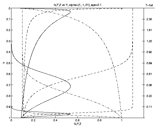
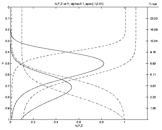
are illustrated on Figure 1. As time progresses P grows,
eventually achieving a maximum (Pm at ym where
Nm = Zm). Subsequently, as the front advances P
decreases, as Z increases towards the sea surface.
The time
at which the front arrives at a given
level is shown on the scale on the right. An interesting
result is that the shapes and subsurface locations of the
nutricline and of the phytoplankton maximum depend
sensitively on the parameter a. For rapid advection
(a = 1, Fig. 1a)
ym = 0.3 whereas for slow advection (a = .01) ym = .97.
The magnitude of Pm depends solely upon the fractional biomass
of seed plankton e. Note (e.g., e = .1 Fig. 1b) a
Pm considerably less than B can mediate the
conversion of almost the entire biomass to Z. Analytically,
|
hm = |
é
ę
ë
|
|
e3
(1-e)(1-e2)
|
ů
ú
ű
|
1/2
|
ym = hma (6.5c) |
|
|
Nm = Zm = [e(1+e)]1/2 Pm = 1+2{e-[e(1+e)]1/2}. |
|
In general, for uniform deep reservoirs with b = 1 it can be
shown that
|
Nm = Zm = (N0Z0)1/2 Pm = N0+P0+Z0-2(N0Z0)1/2 (6.6) |
|
Thus the sensitivity is primarily related to the
amount of seed zooplankton. Although this is a very
simple example, the results indicate the potential
applicability of the theory to important phenomena
including deep chlorophyll maxima (Parsons, op. cit.) and
zooplankton control of blooms (Steele and Henderson, 1995).
This mid-depth phytoplankton bloom Pm is of course
dynamically analogous to the temporal bloom, e.g., the
solution given by equation (I.4.12).
Figure 1. Profiles of N (dot-dash), P (solid), Z (dash)
versus depth. Dependencies upon: (a) advection for fixed
e = 0.1, (a = 1: upper Pm, a = 0.1: middle Pm,
a = 0.01: lower Pm); (b) seed plankton for fixed a = 0.1
(e = 0.1: larger Pm, e = 0.01: smaller Pm).
Nm=Zm at Pm identifies the associated curves. The
scale to the right of (1a) is for a = 1; for a = 0.1 (0.01)
multiply by 10 (102).
(c) Deep Nutricline
Now consider the case that at t = 0 nutrient increases linearly
with depth from zero at the base of the euphotic zone to
unity at a nondimensional depth (H) in the
aphotic zone. We retain the assumptions of no x-dependence,
no nutrient in the euphotic zone initially in time, and
a uniform deep reservoir of seed phytoplankton. Thus
|
y < 1 N(y,0) = 0; y > 1 N(y,0) = |
é
ę
ë
|
(y-1)
H-1
|
ů
ú
ű
|
, (6.7a) |
|
and
|
y Ł 1 N0 = |
é
ę
ë
|
yeat-1
H-1
|
ů
ú
ű
|
P0 = e, (6.7b) |
|
for solution to equation (4.3) following the
arguments of equation (6.1). The dependencies upon
the parameters a,e,d has been
studied numerically with l = 1-y. The results
are summarized on Figure 2 for the case H = 2
such that N0(y = 2,t = 0) = 1. The greatest sensitivity
is again related to a. The important result
here is the existence of a subsurface maximum of
phytoplankton (Pm) in the absence of grazing
loss to zooplankton. At
any given time
, the water in the
vicinity of
entered the
euphotic zone with negligible nutrient. The water
just above y = 1 has been illuminated at a low light
level and for only a short time. Thus the mid-depth
Pm. The existence of subsurface phytoplankton
maxima in this theory will in general be due both to this
dynamical process and that of the preceding paragraph.
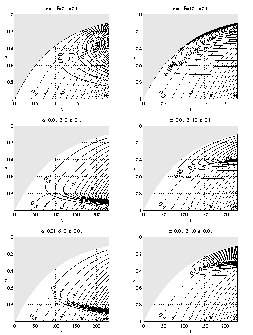
Figure 2. Isolines of N (dashed), P (solid) in the y-t
plane as a function of a,d,e. The dynamically
inert upper euphotic zone is shaded.
Finally spatial localization is illustrated by
the solution of this problem with idealized
coastal upwelling kinematics (LS flow). Figure 3
shows sections (xy plots) of phytoplankton
concentration for as a function of
a,e,d also with l = 1-y
and H = 2. These plots are for the last time
shown on the corresponding plots of Figure 2.
The P(y) at x = 0 on Figure 3 are
thus identical to the final profiles of
Figure 2. The front is advancing as
|
|
^
y
|
= [1+e-[^(x)](ea[^(t)]-1)]-1 (6.8) |
|
Note the development of two-dimensional
subsurface phytoplankton distributions which
can be described as subsurface patches
extending along the front. Subsurface
patches of chlorophyll are features common
to many fronts (Franks and Walstad, 1997).
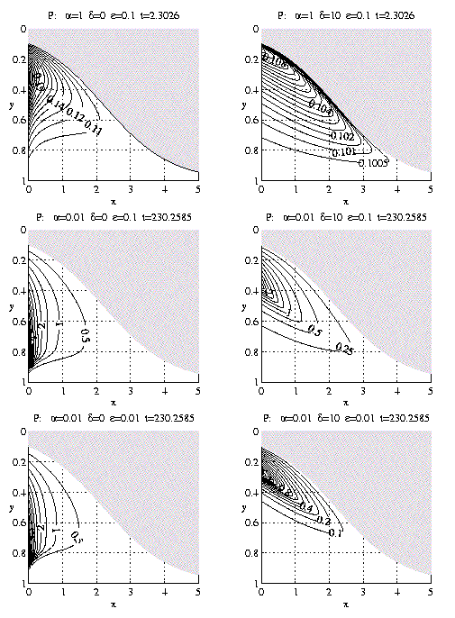
Figure 3. As in Figure 2 for P but in the y-x plane for
fixed t as indicated.
7. Summary and Conclusions
A general theoretical solution has been obtained
for a model ocean in which a dynamically active near-surface
euphotic zone overlies a deeper region in which
biological material is passively advected by
the physical flow field. Illustrative dynamical
solutions have been presented in one-to-three state
variables for an NPZ-model in which nutrient
uptake is nonlinearly modeled by
Michaelis-Menten kinematics. Parametric
dependencies are represented in terms of
four nondimensional parameters: i) the ratio
of the nutrient uptake rate to the advection
rate (a); ii) the ratio of the
zooplankton grazing rate to the uptake rate (b);
iii) the ratio of biomass to the saturation constant
(d); and iv) the ratio of the seed
plankton biomass to nutrient mass in the
aphotic zone (e). A sensitivity
analysis has been initiated. Interesting results
are indicated for the location, shape and magnitude of
phytoplankton maximum and associated
nutricline in the euphotic zone, and for the
dynamical mechanism by which phytoplankton mediate the
conversion of nutrient to zooplankton biomass. For
general biological dynamics kinematical flow
fields have been introduced representative
of coastal upwelling, isolated open ocean eddies
and wave fields; and upwelling events which
set-up in time over a finite time interval.
Explicit solutions for the associated family of
characteristic curves have been obtained.
These results provide a theoretical framework for
further studies of more realistic oceanic
processes. Weak background mixing in the lower
euphotic zone will merely provide some smoothing of
the solutions. For the upper euphotic zone,
a mixed layer model has been added to the model.
Work is in progress extending the model to include
zooplankton mortality (Steele and Henderson, 1990).
Interesting application areas include
mesoscale eddy nutrient injection events
(McGillicuddy et al., 1998), wind-driven
upwelling events
(Franks and Walstad, 1997)
equatorial upwelling (Murray et al., 1995) and
spring blooms (Fasham, 1995).
Acknowledgments
I am grateful to Drs. Patrick J. Haley Jr. and Dennis
J. McGillicuddy, Jr.
for interesting scientific discussions and
comments. It is a pleasure to acknowledge the general
assistance in carrying out this researcch of Mr. Wayne G.
Leslie, who together with Dr. Haley performed
computations and prepared figures. I thank Drs. Dimitri
Kroujiline and Pierre F.J. Lermusiaux for helpful
comments on the manuscript, and Ms. Gioa Sweetland
and Mrs. Renate D'Arcangelo for preparation of the manuscript.
This research was supported in part by the Office of
Naval Research under grant N00014-95-1-0371 to Harvard University.
References
Fasham, M.J.R. 1995 Variations in the seasonal cycle of biological
production in subarctic oceans: A model sensitivity analysis. Deep-Sea Res.,
42, 1111-1149.
Franks, P.J.S. & Walstad, L.J. 1997 Phytoplankton patches at fronts:
a model of formation and response to wind events. J. Mar. Res.,
55, 1-29.
Kirk, J.T.O. 1994 Light & photosynthesis in aquatic
ecosystems, Cambridge: Cambridge University Press.
McGillicuddy, D.J., Robinson, A.R., Siegel, D.A., Jannasch, H.W.,
Johnson, R., Dickey, T.D., McNeil, J., Michaels, A.F. & Knap, A.H. 1998
Influence of mesoscale eddies on new production in the Sargasso Sea.
Nature, 394, 263-265.
Murray, J.W., Johnson, E. & Garside, C. 1995 A U.S. JGOFS
Process Study in the Equatorial Pacific (eqPac): Introduction.
Deep-Sea Research, 42 (2-3), 275-293.
Parsons, T.R., Takahashi, M. & Hargrave, B. 1984
Biological oceanographic processes, Oxford and New York:
Pergamon Press.
Robinson, A.R. 1997 On the theory of advective effects on
biological dynamics in the sea. Proc. R. Soc. Lond., A,
453, 2295-2324.
Steele, J.H. & Henderson, E.W. 1992 The role of predation in
plankton models. J. Plankton Res., 14, 157-172.
Steele, J.H. & Henderson, E.W. 1995 Predation control of plankton
demography. J. Mar. Sci., 52, 565-573.
Tritton, D.J. 1988 Physical fluid dynamics, Oxford and New York:
Oxford University Press.
Table 1. Kinematic Flows
-
|
|
|
| Designation | Structure |
|
|
|
| DS | Steady Upwelling |
| DE | Upwelling Event |
| LS | Steady Coastal Upwelling |
| LE | Coastal Upwelling Event |
| WS | Steady Wave or Eddy Field |
| WE | Wave or Eddy Event
|
|
|
|
|
Table 2. Characteristics
|
|
| Flow | s | p | r | q
|
|
|
|
| DST | t | 0 | xe-at | yeat |
|
|
| DSB | t-p |
| xy | 1 |
|
| DET | t |
| xe-aFE0 | yeaFE0
|
|
|
| DEB | t-p |
| xy | 1
|
|
|
| LST | t | 0 | ln[1+e-at(ex-1)] | y[1+e-x(eat-1)]
|
|
|
| LSB | t-p |
| -ln[1-y(1-e-x)] | 1
|
|
|
| LET | t |
| ln[1+e-aFE0(ex-1)] | y[1+e-x(eaFE0-1)]
|
|
|
| LEB | t-p |
|
1
w
|
cos-1 |
ě
í
î
|
coswt+ |
w
a
|
ln[ex(1/y-1)+1] |
ü
ý
ţ
|
|
| -ln[1-y(1-e-x)] | 1
|
|
|
| WST | t | 0 | 2tan-1[e-attanx/2] | y/2[eat(1+cosx)+e-at(1-cosx)]
|
|
|
| WSB | t-p |
| t- |
1
a
|
ln |
é
ę
ë
|
1+(1-y2sin2x)1/2
y(1+cosx)
|
ů
ú
ű
|
|
| sin-1(ysinx) | 1
|
|
|
| WET | t |
| 2tan-1[e-aFE0tanx/2] | y/2[eaFE0(1+cosx)+e-aFE0(1-cosx)]
|
|
|
| WEB | t-p |
|
1
w
|
cos-1 |
ě
í
î
|
coswt+ |
w
a
|
ln |
é
ę
ë
|
1+(1-y2sin2x)1/2
y(1+cosx)
|
ů
ú
ű
|
ü
ý
ţ
|
|
| sin-1(ysinx) | 1
|
|
|
|
Table 3 Light Attenuation
-
|
|
|
| Flow | y(s;p,r,q) |
|
|
|
| D | qe-aF F = F(s,p)
|
|
| L | q[e-aFe-r+(1-e-r)]
|
|
| W |
| q |
sinr
2
|
[ e-aFtanr/2+e aFtanr/2]
|
|
|
|
|
|
Footnotes:
1 the effects
of environmental conditions upon biological rates.
2 This notation
is equivalent to equation (I.2.13) but simpler.
3 These idealized
dependencies yield simpler analytical solutions than the more
accurate exponential decay which can be treated later.
File translated from TEX by TTH, version 2.51.
On 5 Oct 1999, 17:02.